
We derive the math, write it in pure Python, then watch scikit-learn do the same in two lines. Spoiler: the results are identical.
In the last post, I explained what ML is — pattern recognition at scale. Today we stop talking about it and actually build something. Our first real ML model: Linear Regression.
I’ll be honest — when I first heard “linear regression”, I assumed it was some advanced stats technique only academics care about. Turns out it’s the foundation of almost everything in ML, and once you understand it, a huge chunk of the field starts clicking.
Let’s go from zero to working model — math first, then code.
The intuition: drawing the best possible line
Remember the scatter plot from last post? House size on the x-axis, price on the y-axis, a cloud of dots. Linear regression answers one question: what is the best straight line I can draw through this cloud?
That line lets you predict. Given a new house size you’ve never seen, you find that x-value on the line, read off the y-value, and that’s your predicted price. Simple — but incredibly powerful.
The word “linear” just means straight line. “Regression” means we’re predicting a continuous number (like price), not a category. That’s it. Don’t let the name intimidate you.
The math — let’s derive it
A straight line has the equation:
THE LINE EQUATION
Our model’s job is to find the right values of w and b. But how do we know if a line is “good”? We measure error.
Step 1 — measure the error with MSE
For every data point, our line makes a prediction. The prediction will be wrong by some amount. We square those errors and average them — this is called Mean Squared Error:
LOSS FUNCTION – MEAN SQUARED ERROR
We square the errors so negatives don’t cancel positives, and so big errors are punished more. Our goal is to find the w and b that make MSE as small as possible.
Step 2 — the closed-form solution
For linear regression, we’re lucky — we don’t need to guess. There’s an exact formula (derived by setting the derivative of MSE to zero and solving):
OPTIMAL WEIGHT AND BIAS – EXACT SOLUTION
This looks scary. But it’s just arithmetic. Let’s turn it into Python.
How much x and y move together ÷ how much x varies
Pure Python implementation
No libraries. Just Python and math. This is the real thing:
PYTHON – LINEAR REGRESSION FROM SCRATCH
import numpy as np
import matplotlib.pyplot as plt

# Generate some fake "house size vs price" data
np.random.seed(42)
x = np.random.randint(500, 3500, 50).astype(float)          # sq ft
y = x * 150 + np.random.randn(50) * 30000  # noisy relationship


# Mean Calculation
x_mean = np.mean(x)

y_mean = np.mean(y)

# Slope Calculation

# w = sum((x-x_mean) * (y-y_mean))/sum((x-x_mean)^2)

numarator = np.sum((x-x_mean) * (y-y_mean))
denominator = np.sum(np.square(x-x_mean))

w = numarator/denominator # slope

# b = y_mean * w - x_mean

# Intercept Calculation

b = y_mean - (w * x_mean) # intercept

print(f"slope(w) {w:.2f}")
print(f"intercept(b) {b:.2f}")

y_pred = w * x + b# --- evaluate ---
mse = np.mean((y - y_pred) ** 2)
print(f"MSE: {mse:.2f}")

# --- plot ---
plt.scatter(x, y, alpha=0.6, label="actual data")
plt.plot(x, y_pred, color="red", label="our model")
plt.xlabel("House size (sq ft)")
plt.ylabel("Price ($)")
plt.legend()
plt.title("Linear Regression — from scratch")
plt.show()slope(w) 156.23
intercept(b) -10850.87
MSE: 877663111.31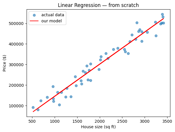
Interactive linear regression explorer — drag sliders to adjust slope and intercept and see how the line fits the data
A few things worth noticing about this lesson:
The interactive explorer is the star of this post. Drag the slope and intercept sliders and watch your line move against the scatter plot — the blue dashed line is always the mathematically perfect fit. That gap between "your MSE" and "best MSE" is exactly what the learning algorithm is trying to close. No textbook explains this as viscerally as playing with it yourself.
What's coming in Lesson 3 — Gradient Descent: The closed-form solution works perfectly for linear regression, but it breaks down the moment your data has millions of rows or hundreds of features. Gradient descent is the general-purpose algorithm that solves this — and it's the beating heart of neural networks, deep learning, and everything in modern ML. We'll build it visually first (literally rolling a ball down a hill), then in code.