Gradient Descent: the engine that powers all of modern ML

We couldn’t always use a formula to find the best model. Here’s the algorithm that solves that — and it’s the same one powering GPT, Stable Diffusion, and everything in between.

In the last post, we found the perfect slope and intercept for our linear regression model using a neat closed-form formula. Plug in the numbers, out comes the answer. Done.

But I kept wondering: what happens when there’s no clean formula? What if we have thousands of parameters instead of two? What if the math doesn’t simplify nicely?

That’s exactly the problem gradient descent solves. And it turns out to be the most important algorithm in all of machine learning.

The hill analogy — seriously, it works

Imagine you’re blindfolded on a hilly landscape, and your goal is to find the lowest point in the valley. You can’t see the whole landscape — you can only feel the slope beneath your feet right now.

What do you do? You take a small step in whichever direction goes downhill. Then check the slope again. Step downhill again. Repeat until you’re not going downhill anymore — you’ve found the bottom.

That’s gradient descent. The “landscape” is your loss function (MSE). The “lowest point” is the best possible model. Each “step” is an update to your model’s parameters. The “slope beneath your feet” is the gradient — a mathematical measure of how steep the loss is right now.

The beauty of this: it works even when you have millions of parameters. No formula needed — just keep stepping downhill.

The math — one update rule to rule them all

For our linear regression with one feature, here’s exactly how we update w and b at each step:

For MSE loss, the gradients work out to:

Don’t panic at the calculus notation. In plain English: the gradient is just a measure of “if I nudge w slightly, how much does my loss go up or down?” We subtract it — because we want to go down.

The learning rate — the most important hyperparameter
The learning rate α controls how big each step is. Too large and you overshoot the valley floor and bounce around. Too small and it takes forever to get there. Picking a good learning rate is one of the first real skills you develop as an ML practitioner.

Pure Python implementation

Here’s gradient descent from scratch — every step visible, nothing hidden:

PYTHON – GRADIENT DESCENT FROM SCRATCH

import numpy as np
import matplotlib.pyplot as plt

# 1. Generate data
np.random.seed(42)
X = np.random.randint(500, 3500, 50).astype(float)
y = X * 150 + np.random.randn(50) * 30000
n = len(X)

# 2. Normalize X so learning rate works cleanly
X_norm = (X - X.mean()) / X.std()

# 3. Initialize parameters
w, b = 0.0, 0.0
lr = 0.01          # works well on normalized data
epochs = 300
losses = []

# 4. Gradient descent loop
for epoch in range(epochs):
    y_pred = w * X_norm + b        # forward pass
    loss = np.mean((y - y_pred) ** 2)   # MSE loss
    losses.append(loss)

    dw = (2/n) * np.sum((y_pred - y) * X_norm)   # gradient of w
    db = (2/n) * np.sum(y_pred - y)               # gradient of b

    w -= lr * dw   # update w
    b -= lr * db   # update b

    if epoch % 50 == 0:
        print(f"Epoch {epoch:3d} | Loss: {loss:>15,.0f} | w={w:8.2f} | b={b:10.2f}")

# 5. Plot loss curve
plt.figure(figsize=(8, 4))
plt.plot(losses, color='#1D9E75', linewidth=2)
plt.xlabel("Epoch")
plt.ylabel("MSE Loss")
plt.title("Loss curve — gradient descent converging")
plt.tight_layout()
plt.show()

print(f"\nFinal w: {w:.4f}, b: {b:.2f}")

import numpy as np
import matplotlib.pyplot as plt

# 1. Generate data
np.random.seed(42)
X = np.random.randint(500, 3500, 50).astype(float)
y = X * 150 + np.random.randn(50) * 30000
n = len(X)

# 2. Normalize X so learning rate works cleanly
X_norm = (X - X.mean()) / X.std()

# 3. Initialize parameters
w, b = 0.0, 0.0
lr = 0.01          # works well on normalized data
epochs = 300
losses = []

# 4. Gradient descent loop
for epoch in range(epochs):
    y_pred = w * X_norm + b        # forward pass
    loss = np.mean((y - y_pred) ** 2)   # MSE loss
    losses.append(loss)

    dw = (2/n) * np.sum((y_pred - y) * X_norm)   # gradient of w
    db = (2/n) * np.sum(y_pred - y)               # gradient of b

    w -= lr * dw   # update w
    b -= lr * db   # update b

    if epoch % 50 == 0:
        print(f"Epoch {epoch:3d} | Loss: {loss:>15,.0f} | w={w:8.2f} | b={b:10.2f}")

# 5. Plot loss curve
plt.figure(figsize=(8, 4))
plt.plot(losses, color='#1D9E75', linewidth=2)
plt.xlabel("Epoch")
plt.ylabel("MSE Loss")
plt.title("Loss curve — gradient descent converging")
plt.tight_layout()
plt.show()

print(f"\nFinal w: {w:.4f}, b: {b:.2f}")

Epoch 0 | Loss: 115,099,184,524 | w= 2661.83 | b= 6213.15 
Epoch 50 | Loss: 16,025,670,555 | w=85592.93 | b= 199788.21 
Epoch 100 | Loss: 2,886,585,131 | w=115793.92 | b= 270282.38 
Epoch 150 | Loss: 1,144,085,457 | w=126792.21 | b= 295954.22 
Epoch 200 | Loss: 912,995,925 | w=130797.45 | b= 305303.12 
Epoch 250 | Loss: 882,348,933 | w=132256.04 | b= 308707.71 
Epoch 300 | Loss: 878,284,543 | w=132787.21 | b= 309947.56 
Epoch 350 | Loss: 877,745,525 | w=132980.65 | b= 310399.07 
Epoch 400 | Loss: 877,674,041 | w=133051.09 | b= 310563.50 
Epoch 450 | Loss: 877,664,561 | w=133076.74 | b= 310623.38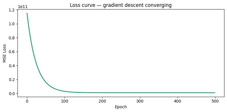

Final w: 133085.9769, b: 310644.93

Graph After Gradient Descent

# Now Let's Verify the MSE
mse = np.mean((y - y_pred) ** 2)
print(f"MSE: {mse:.2f}")

# --- plot ---
plt.scatter(X_norm, y, alpha=0.6, label="actual data")
plt.plot(X_norm, y_pred, color="red", label="our model")
plt.xlabel("House size (sq ft)")
plt.ylabel("Price ($)")
plt.legend()
plt.title("Linear Regression — after Gradient descent")
plt.show()

# Now Let's Verify the MSE
mse = np.mean((y - y_pred) ** 2)
print(f"MSE: {mse:.2f}")

# --- plot ---
plt.scatter(X_norm, y, alpha=0.6, label="actual data")
plt.plot(X_norm, y_pred, color="red", label="our model")
plt.xlabel("House size (sq ft)")
plt.ylabel("Price ($)")
plt.legend()
plt.title("Linear Regression — after Gradient descent")
plt.show()

MSE: 877663311.46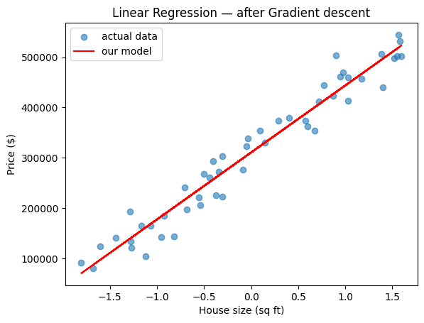

Why not always use the closed-form solution?

Great question. For simple linear regression with one feature, the formula from last post is perfect — fast and exact. But gradient descent wins when:

1. You have millions of data points — the closed-form formula requires inverting a matrix, which becomes impossibly expensive at scale.

2. You have complex models — neural networks have billions of parameters. There’s no formula for their optimal values. Gradient descent is the only way.

3. You need flexibility — gradient descent works with any differentiable loss function, not just MSE.

This is why gradient descent is everywhere. It’s not the fanciest algorithm — it’s just the one that scales. Every neural network, every LLM, every image generator you’ve heard of was trained with some variant of gradient descent.

Variants you’ll encounter

What we built above is called Batch Gradient Descent — we use all data every step. In practice, two variants are more common. Stochastic Gradient Descent (SGD) uses one random sample per step — noisy but fast. Mini-batch Gradient Descent uses a small batch (32–256 samples) — the sweet spot used in almost all real training today.

What I learned today

Gradient descent is beautifully simple: compute how wrong you are, figure out which direction makes things worse, go the other way. Repeat. That loop — forward pass, compute loss, compute gradient, update — is the heartbeat of every ML model ever trained.

Next up: our first real project — a spam classifier built with everything we’ve learned so far. We’ll go from raw data to a working model you can test with your own emails.

Lesson 4 is where things get exciting — we’ll use everything learned so far to build a working spam classifier on real email data, from raw text all the way to predictions. Full blog post format as always.